How neural networks learn: margin maximisation

A partial answer regarding how neural networks generalise

While the mystery of how neural networks can learn so well is not fully understood, some progress has been made in explaining why gradient descent can find solutions that generalise well. Margin-maximisation is an example of such progress; a theoretical result that shows that gradient descent, in some cases, converges to solutions with properties that could conceivably be related to good generalisation. In this post, I provide an overview of what has been discovered so far, and some questions that remain open.

First, some bad news: these results are pretty restricted. For example, they probably don’t apply directly to frontier models like transformers. Several assumptions are required.

One of these assumptions is that the learning task at hand is a classification task. That is to say, we have data belonging to several classes (such as images of different animals), along with labels stating which class each datapoint belongs to. For simplicity, let’s stick to the case with only two classes (binary classifcation - but everything here can be generalised to multiclass classification). For example, our two classes could be images of vehicles and images of animals.

The second restriction we’ll make is to focus on homogenous neural networks and loss functions with exponential tails. Homogeneity essentially means that the behaviour of the neural network depends only on the direction (and not the magnitude!) of the parameter vector. As for exponentially-tailed loss functions, many common loss functions satisfy this property (such as logistic loss, exponential loss, and binary cross-entropy). For definitions of these terms, see appendix A of this paper.

For simplicity, we will assume that our neural network outputs a single scalar value. We train the network to output a positive value for one class, and a negative value for the other class. We will call the classes the positive and negative classes respectively.

Given these assumptions, we have some good news: an existing result about the linear classification can be extended to deep neural networks to say something fairly precise about where gradient descent converges.

The existing result: linear classification

Soudry et al answer a simpler question: what happens in the setup described if the classifier is linear (i.e., prediction is done simply by taking the dot product with a classifier vector)? In the 2D case this looks like finding a line (passing through the origin) that separates the two data classes.

Two possible separating lines

This question is interesting when the classification problem is underdetermined: multiple lines can separate the data. For example, lines A and B above both separate the red and blue points. Can we say which line will be selected by gradient descent?

Yes, as it turns out! If we have our assumptions (exponential-tailed loss function, separability of the datapoints - homogeneity is implied by linearity of the classifier). In particular, we have convergence to the maximum-margin classifier, the one that separates the points while leaving as much space between the decision boundary and the points as possible. Hence line B would be selected and not line A, as line B is the maximum-margin separating line.

Extending to neural networks

Lyu and Li show that gradient descent on neural networks has a similar property when our assumptions hold. To explain the result, we first need to generalise some concepts from linear classification to homogeneous neural networks.

Separability

Our separability assumption will be stronger than in the case of linear classification. Instead of just assuming that there exists a parameter value for which the neural network separates the class, we assume that gradient descent finds such a parameter value. That is, there exists a training step with 100% accuracy on the training dataset.

Margins in parameter space

Perhaps the most obvious way to extend the concept of the margin to neural networks is to simply ask what is the minimum (euclidean) distance between a datapoint and the decision boundary. This is referred to as the margin in function space.

Lyu and Li’s result uses a different concept; the parameter space maximum-margin. They consider the margin for a model that separates the dataset to be the minimum over all inputs of the absolute value of the model’s output. Intuitively, if the function implemented by the neural network is not too steep then high output value means that the datapoint is probably not very close to the decision boundary, as shown below:

If the neural network implements a continuous function, a larger output means greater distance from the decision boundary

Now, we use this definition of the margin to formulate our notion of the maximum margin. Remember that our neural network is homogeneous, so you can find solutions with arbitrarily high margin just by scaling up the parameter! Therefore, we focus only on the unit sphere in parameter space. Now we can state the optimisation problem that defines the parameter-space maximum-margin solutions:

\(\max_{\mathbf{\theta}\in\mathbb{R}^p, |\mathbf{\theta}|=1}\gamma(\mathbf{\theta})\)

where theta represents the parameter, and gamma is the margin.

The result

Now, it would be nice if we had a result saying that gradient descent causes the parameter vector to converge to the direction of a maximum-margin solution. Instead we have something close. Lyu and Li prove that every limit point of gradient descent is in the direction of KKT point of the maximum-margin problem optimisation problem. (Ji and Telgarsky strengthen the result, showing that convergence in direction always happens, and we do not need to speak about limit points.)

This means that, in the infinite limit of training time, the parameter vector will satisfy an equation: it is a linear combination of the of the gradients of the neural network with respect to the parameter vector at each datapoint:

\(\mathbf{\theta}=\sum_{i=1}^n\lambda_i\nabla_{\mathbf{\theta}}\Phi(\mathbf{\theta}; x_i)\)

Here, λ_i is a positive constant for datapoints x_i in the positive class, and is negative for datapoints x_i in the negative class. Φ is a parametrisation of the neural network.

Being a KKT point is a necessary condition for being the maximum, but it’s not sufficient here. Vardi et al. (2022) goes as far showing that sometimes a neural network’s parameter vector can be a KKT point without even being a local maximum of this margin-maximisation problem!

So what does this mean for margin-maximisation as an explanation of gradient descent? Well, empirically the margin increases throughout training, so there does seem to be something to the result. And in even more restricted settings, there are results showing that the global maximum is in fact reached; Chizat and Bach is one such result, for infinite-width networks.

What can we do with the result?

As we’ve seen, the result seems pretty limited.

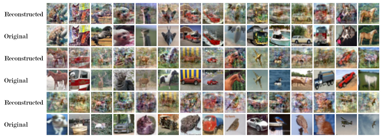
And yet, despite the limitations, at least one paper uses it to achieve almost breath-taking results. Haim et al. (2022) reconstruct the training data of a neural network from its parameters. The key insight that enables this is that the KKT equation above essentially has two unknowns: the dataset, and the parameter vector. Just as it gives information about the parameter vector in terms of the dataset, it can also tell you about the training dataset in terms of the parameters!

Some training data reconstructed by Haim et al., from a network trained to classify images as vehicles or animals

I think that this shows that margin-maximisation is a pretty high-leverage result: you can use it to do pretty non-trivial things, despite its apparent weakness! The caveat here is that it requires training the neural network under somewhat contrived conditions: you need no biases, and small initialisation to ensure that the limit is reached.

Another possible application of the result is to predict what features a neural network might learn. For example, it has been used to show that the features found by Chughtai et al. (2032) in a neural network trained to perform modular addition are present in maximum-margin solutions.

Sources

I was helped a lot in writing up this post by Vardi (2023)’s excellent review of results about implicit bias.